
Often data within an Excel file will be displayed in a classic (pivot) table format, with a defined two dimensional layout of rows and columns. The rows and columns usually have associated headers/titles and the data within the table may be a summary of some underlying source data using sums or averages.
This data table format is recognised by most users and can make reading and interpretation of the data easier, particularly when looking at values at the intersection of rows and columns. However, working with this type of data, particularly if looking to filter or group the data, can be more difficult.
A common approach within data analysis is to look to un-pivot (or “flatten”) such data tables into a single vertical data table where each row represents a data point and the columns contain the attributes for that data point — data structures such as seen in relational databases or Power Query.
By unpivoting your data into this kind of structure, analysis is easier, especially when applying filtering to the data. The unpivoted data table can also act as a single main data source for any output calculations or charts/visualisations, so that when applying filtering to this one data source it will then be reflected in all outputs that are linked to that data.
For example, with the data shown below, when charting the sales per quarter for a chosen region you could simply use a look-up formula such as XLOOKUP() based on the region required. However, if you wanted to show a detailed comparison by region for a specified quarter then either different look-up formula logic is needed, or a more complex and less efficient formula is requried to allow for both situations dynamically.


If instead, the same data is unpivoted to a flat vertical data table where each row is a single data point and columns are present for region, quarter and year, then simple filtering logic could be used to show either sales across quarters for a specified region or regional performance over a specified quarter, and the change between the two can easily be accomplished.
This data structure also allows for easy interactivity with Slicers and can fairly easily facilitate cross-filtering of an output with multiple Slicers as seen with Power BI style dashboards.

Achieving this kind of unpivoted data table is simple when done manually but can be time consuming and will need updating when the underlying data changes. Alternatively, a more dynamic approach to the unpivoting could be achieved using look-up formulae, but this would likely need manually updating if the structure of the underlying data table is changed, e.g. if rows or columns are added/removed in the underlying data table.
Power Query, once setup, provides a good way to achieve a fully dynamic approach to unpivoting worksheet data whilst allowing for structural and data changes, but requires refreshing of the query for the worksheet output to reflect any source data changes.
This is what inspired me to use a dynamic array-based approach with a custom LAMBDA() function to achieve a fully dynamic and flexible solution to unpivoting my data as standard Excel formulae on the worksheet.
UnPivot() Function
The UnPivot() function takes a two-dimensional (2D) array of data points/values (data input parameter) along with inputs for the associated row headers/labels and columns headers/labels (row_headers & column_headers input parameters). The data points in the main data array are converted to a single column of values and are displayed with the associated row and column headers for each data point. In this way each data point from the source table has its own row and has the useful associated information on the same row in columns next to the data values column.
The row and column header input arrays can be a single row/column or multiple rows/columns allowing for more detailed labelling of each data point and providing more columns on which any filtering or grouping can be applied.
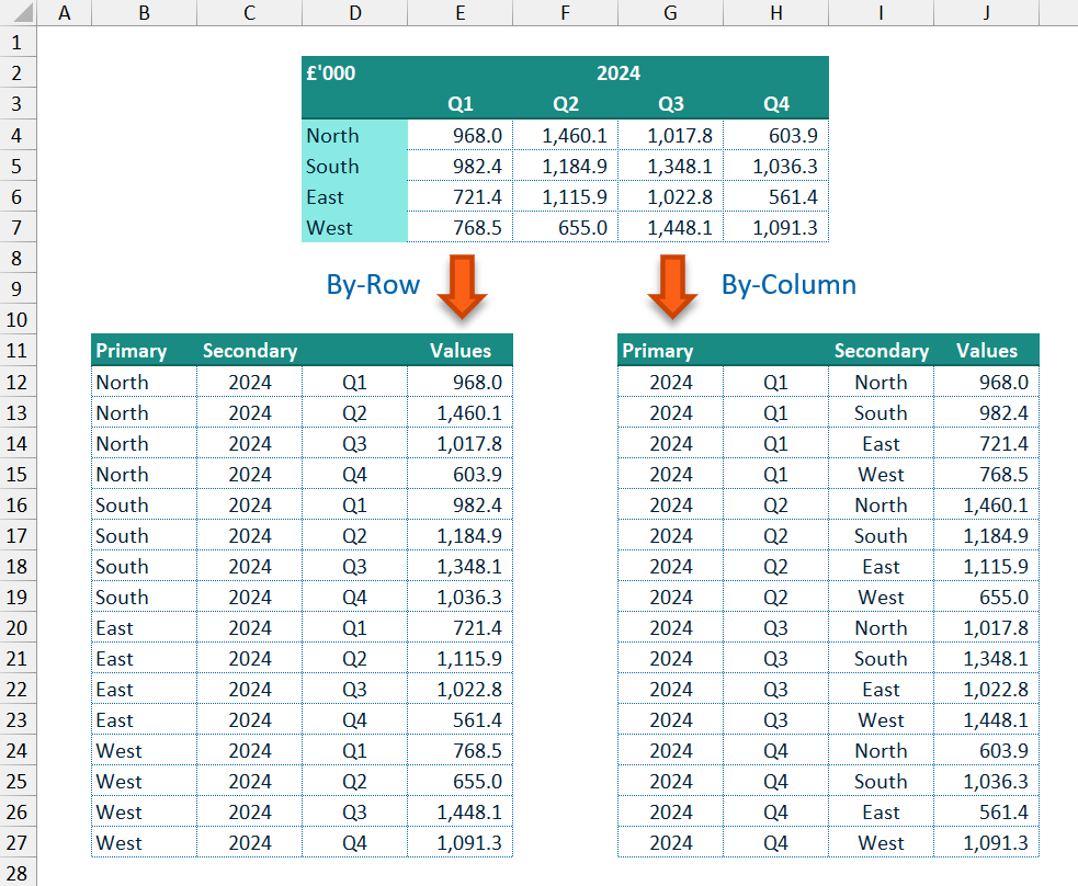
The cells in the data array can be read in a by-row manner (across each row left-to-right) or a by-column manner (down each column top-to-bottom). By default, the data array is read by-row, and the row headers are used as the primary (“Key”) associated label column(s) with the column headers as the secondary (“Name”) label column(s). If the data array is read by-column instead (via the by_column input parameter), then the column headers are used as the primary “Key” column(s) and the row headers as the “Name” column(s).
To make the function more flexible, blank values in the input arrays can be filled or replaced. With the main data array, the replace_data_blanks input parameter can be used to provide a new value, such as a 0 (zero), which is used to replace any blank data points. For the row and column headers, replacing blank values is more complicated. The function allows the user to fill any blank values:
- in the
row_headersarray with values from the row above or below (via thefill_row_blanksinput parameter); and - in the
column_headersarray with values from the column to the left or the right (via thefill_column_blanksinput parameter).
Filtering can also be applied to the final output to remove any rows where the data values column contains blank cells or Excel error cells, using the filter_blanks and filter_errors input parameters.
Function code
= LAMBDA(
  // Parameter definitions
  data,
  row_headers,
  column_headers,
  [by_column],
  [replace_data_blanks],
  [filter_blanks],
  [filter_errors],
  [fill_row_blanks],
  [fill_column_blanks],
  [output_vertical],
  // Main function body/calculations
  LET(
    _dd, data,
    _rh, row_headers,
    _ch, column_headers,
    // Dealing with default values for optional parameters
    _byCol, IF( ISOMITTED(by_column), 0, IF(by_column, 1, 0)),
    _repD, IF( ISOMITTED(replace_data_blanks), "",
      IF( ISLOGICAL(replace_data_blanks),
        IF(replace_data_blanks, NA(), ""),
        replace_data_blanks)
    ),
    _fltrB, IF( ISOMITTED(filter_blanks), 0, IF(filter_blanks, 1, 0)),
    _fltrE, IF( ISOMITTED(filter_errors), 0, IF(filter_errors, 1, 0)),
    _rowB, IF( ISOMITTED(fill_row_blanks), 0, fill_row_blanks),
    _colB, IF( ISOMITTED(fill_column_blanks), 0, fill_column_blanks),
    _vrt, IF( ISOMITTED(output_vertical), 1, IF(output_vertical, 1, 0)),
    // Determine the correct fill direction and if a replacement is string is needed
    // for both the row_headers and column_headers input arrays
    _repR, IF( OR(ISNUMBER(_rowB), ISLOGICAL(_rowB)), "", _rowB),
    _repC, IF( OR(ISNUMBER(_colB), ISLOGICAL(_colB)), "", _colB),
    _dirR, IF( OR(ISNUMBER(_rowB), ISLOGICAL(_rowB)), INT(_rowB), 0),
    _dirC, IF( OR(ISNUMBER(_colB), ISLOGICAL(_colB)), INT(_colB), 0),
    // Input parameter checks
    _inpChk, IFS(
      IFERROR( OR( ROWS(_rh) < 1, COLUMNS(_rh) < 1, ROWS(_ch) < 1, COLUMNS(_ch) < 1, ROWS(_dd) < 1, COLUMNS(_dd) < 1), 3), 3,
      IFERROR( OR( ROWS(_dd) <> ROWS(_rh), COLUMNS(_dd) <> COLUMNS(_ch)), 3), 2,
      TRUE, 1
    ),
    // Assign the row header and column header input arrays to the key columns and name columns arrays depending on the by_column input
    // ensure that assigned key and name column arrays are vertically aligned
    // get the dimensions (rows, columns) of the assigned arrays
    _kCols, IF(_byCol, TRANSPOSE(_ch), _rh),
    _nCols, IF(_byCol, _rh, TRANSPOSE(_ch)),
    _rK, ROWS(_kCols),
    _cK, COLUMNS(_kCols),
    _rN, ROWS(_nCols),
    _cN, COLUMNS(_nCols),
    // Construct the keys (primary) and names (secondary) columns for the output array
    // + The input array is reversed if needed (depending on the direction chosen), and then
    //   a combination of REDUCE(), HSTACK() and SCAN() are used to fill any blanks with an
    //   an appropriate replacement value, one column at a time
    // + The updated input array is returned to it's original direction if needed before being
    //   used in the MAKEARRAY() function to construct the final Keys/Names column.
    _keys, LET(
      _kRep, IF(_byCol, _repC, _repR),
      _kDir, IF(_byCol, _dirC, _dirR),
      _kArr, IF(_kDir = -1, INDEX(_kCols, SEQUENCE(_rK, 1, _rK, -1), SEQUENCE(1, _cK)), _kCols),
      _kFil, DROP( REDUCE(0, SEQUENCE(_cK), LAMBDA(_arr,_col,
        HSTACK(_arr,
          SCAN("", CHOOSECOLS(_kArr, _col),
            LAMBDA(_acc,_val, IF(ISBLANK(_val), IF(_kDir = 0, _kRep, _acc), _val))
          )
        ))),
      , 1),
      _out, IF(_kDir = -1, INDEX(_kFil, SEQUENCE(_rK, 1, _rK, -1), SEQUENCE(1, _cK)), _kFil),
      MAKEARRAY(_rK * _rN, _cK, LAMBDA(_row,_col, INDEX(_out, ROUNDUP(_row / _rN, 0), _col)))
    ),
    _names, LET(
      _nRep, IF(_byCol, _repR, _repC),
      _nDir, IF(_byCol, _dirR, _dirC),
      _nArr, IF(_nDir = -1, INDEX(_nCols, SEQUENCE(_rN, 1, _rN, -1), SEQUENCE(1, _cN)), _nCols),
      _nFil, DROP( REDUCE(0, SEQUENCE(_cN), LAMBDA(_arr,_col,
        HSTACK(_arr,
          SCAN("", CHOOSECOLS(_nArr, _col),
            LAMBDA(_acc,_val, IF(ISBLANK(_val), IF(_nDir = 0, _nRep, _acc), _val))
          )
        ))),
      , 1),
      _out, IF(_nDir = -1, INDEX(_nFil, SEQUENCE(_rN, 1, _rN, -1), SEQUENCE(1, _cN)), _nFil),
      MAKEARRAY(_rK * _rN, _cN, LAMBDA(_row,_col, INDEX(_out, MOD(_row - 1, _rN) + 1, _col)))
    ),
    // Construct the values (data values) column for the output array
    _values, LET(
      _dp, TOCOL(_dd, , _byCol),
      IF( ISBLANK(_dp), _repD, _dp)
    ),
    // Construct the output array
    _rtn, LET(
      _dt, HSTACK(_keys, _names, _values),
      _vl, CHOOSECOLS(_dt, -1),
      // Apply filtering to the constructed output array for blanks and/or errors
      // Note - filtering is only based on the Values (data values) column,
      //        blanks or error values in the Keys and Names columns will not be filtered
      _dfB, IF(_fltrB, FILTER(_dt, IF( ISERROR(_vl), TRUE, IFNA(_vl, "#") <> "")), _dt),
      _dfE, IF(_fltrE, FILTER(_dfB, NOT(ISERROR( CHOOSECOLS(_dfB, -1)))), _dfB),
      // Transpose the output array if needed
      IF(NOT(_vrt), TRANSPOSE(_dfE), _dfE)
    ),
    // Check if input checks have flagged -- if so return the appropriate error, otherwise return the calculated output array
    CHOOSE(_inpChk, _rtn, LAMBDA(0), #VALUE!)
  )
)
The function input parameters are declared in lines 3-12 with the optional parameters defined by the use of square brackets ("[ ]"). This is followed by dealing with the optional parameters setting default values where input values have been omitted (lines 19-29).
Input checks are performed for the three main, and required, input parameters: data, row_headers, and column_headers (lines 37-41).
The main calculated output uses a vertical orientation, i.e. the unpivoted data is converted to a column of data points and output as the “Values” column of the output.
The associated row headers/titles and column headers/titles are assigned to either the primary data column(s) in the output as the “Key” column(s), or the secondary data column(s) in the output as the “Name” column(s). Based on the by_column optional input parameter the user can select whether to unpivot the data by reading down each column of the data array or by default by reading across each row of the data array.
When the by_column option is used, the column headers will make up the primary “Key” columns with the rows as the secondary “Name” columns; otherwise, by default the row headers are used to create the primary “Key” columns and the columns headers used to create the secondary “Name” columns (lines 45-50).
As the unpivoted output array ideally should have no blank values in the “Key” and “Name” columns, the user has the option to fill any blanks via the fill_row_blanks and fill_column_blanks input parameters. The user can choose to:
- provide a new value which is used to fill all blank spaces;
- fill the blank spaces with the value of the cell above (row headers) or to the left (column headers) — input as
True/1; - fill the blank spaces with the value of the cell below (row headers) or to the right (column headers) — input as
-1; or - by default (or an input of
False/0), blanks values are not replaced and instead empty strings ("") are used.
Filling in blank header values with the cell value from the row above/column to the left is relatively simple with a SCAN() function. However, it is more challenging when filling with the cell value from the row below/column to the right. To make this process easier, when constructing the “Key” and “Name” columns, if filling from below/right the input array is first reversed (lines 60 & 74), and then the same SCAN() function logic can be used to fill blanks using the previous non-blank value (lines 61-67 & 75-81), before reverting the array back to its original direction as required (lines 68 & 82).
Once the row and column header arrays have been orientated and updated as required, MAKEARRAY() functions are used to construct the “Key” and “Name” columns (lines 69 & 83). This is used to accommodate 2D input arrays (e.g. multiple columns of row headers, or multiple rows of columns headers), and to allow for the production of an effective Cartesian product to label the unpivoted data array, using a similar logic to that used in the CrossJoin() function (see Data Analysis Tools (1) – CrossJoin Lists).
Having created the “Key” and “Name” columns, the data array is converted to a single column using TOCOL(), reading either by column or by row (line 87), and replacing any blank data points as appropriate (line 88).
The main data values column (_values) and the associated data labelling columns (_keys, _names) are stacked together using a HSTACK() function (line 92). The final output is then be filtered to remove any blank data points or Excel error values in the data values column as needed (lines 97-98), and the orientation of the main output can be changed to horizontal (extending across the worksheet) rather than the default of a vertical output if chosen by the user (line 100).
Finally, the function checks if any of the input checks have flagged (_inpChk), and if so, returns an appropriate Excel error value, otherwise the calculated and filtered output array (_rtn) is returned (line 103).

If you want to use the UnPivot() function in your own projects, I encourage you to include it via the full RXL_Data module. If you would prefer to include just the single function, please use one of the options below:
- Using Excel Labs Advanced Formula Environment (AFE) download the
RXL_UnPivotfunction using the Gist URL https://gist.github.com/r-silk/c31faf1e9de8d01687447bede455f8cc - Alternatively, go to the GitHub repository https://github.com/r-silk/RXL_Lambdas and download the file
RXL_UnPivot.xlsx- this file contains a copy of the function in the Defined Names which can be copied into your own file
- there is also a “minimised” version of the function, however the minimised function string exceeds the number of characters which can be pasted into the “Refers to” text box of the Name Manager window
- instead, you can use the VBA code and instructions on the “VBA” worksheet to copy the function across to your own project using VBA
- the file contains the documentation for the function as well as some details on development and testing/example usage

Leave a comment