Category: Lambdas

Data Analysis Tools (4) – Function Module

In the previous three posts I described some custom LAMBDA() functions which perform actions that can be useful for data analysis: creating a CROSS JOIN product (CrossJoin()), returning the relative position of data points which match a particular search criteria (FindItem()), and unpivoting a table of data to flat-file-style vertical data table (UnPivot).

As such I opted to combine these three functions into a single function module which can be imported to and accessed via the Excel Labs Advanced Formula Environment (AFE).

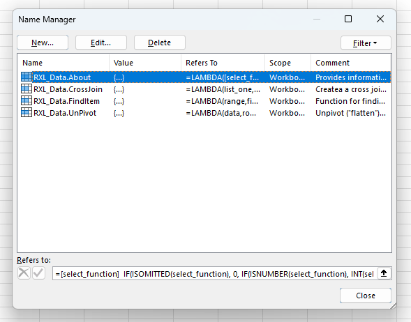
Data Analysis Tools Module (RXL_Data)

Below is the final, combined LAMBDA() module which incorporates an About() function, along with the CrossJoin(), FindItem(), and UnPivot() functions.

The functions are shown in outline only, concentrating instead on the format and structure of the comments, documentation, and definitions. Details on the contents of the module functions can be found in the individual posts for the main three functions (Data Analysis Tools (1) – CrossJoin Lists, Data Analysis Tools (2) – UnPivot Data, Data Analysis Tools (3) – FindItem Function), and details of the About() function can be found in the previous Workbook Information Functions (Part 2).

/*
    MODULE:     RXL_Data
    AUTHOR:     R Silk, RXL Development
    WEBSITE:    https://excel-bits.net
    GIST URL:   https://gist.github.com/r-silk/e66b3b83363166862c83a5246dc1d3ea
    VERSION:    1.03 (May-2025)
*/
/*
    Name:        About()
    Version:     1.10 (23-Apr-2025) -- R Silk, RXL Development
    Description: *//**Provides information about the functions in this module*//*
    Parameters:
        + select_function   = (optional) the name or index number of the function that user wants information about
    Error codes:
        #[Error: name not recognised]   = the provided name string does not match those in the module
        #[Error: index not recognised]  = the provided index number does not match those in the module
    Notes:
        - if the select_function input is omitted or an index of 0 is provided then a table of information about the module is returned
        - the user can either provide the index of the chosen function as an integer (1+), or the name of the chosen function as a string

*/
About = LAMBDA(

    ...

);

/*
    Name:        CrossJoin()
    Version:     1.06 (12-Apr-2025) -- R Silk, RXL Development
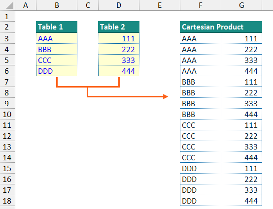
    Description: *//**Createa a cross join (Cartesian join) between two lists; each row of 2nd list is joined to each row of 1st list*//*
                 The provided input lists can be 1D or 2D arrays, and can be vertically or horizontally oriented
                 Where a 2D input array is provided the function can optionally convert this to 1D array/list prior to joining the input lists
    Parameters:
        + list_one              = (required) The 1st input array/list to which the 2nd input array will be joined; should be a valid cell reference
        + list_two              = (required) The 2nd input array/list which is joined to the 1st input array/list; should be a valid cell reference
        + convert_list_one      = (optional) A True/False value which determines whether to convert list_one to a 1D list / a single column list before the join
                                             Will default to FALSE (0) if not supplied
        + list_one_by_column    = (optional) A True/False value -- if list_one is to be converted to a 1D list, this input determines whether to read list_one by column (TRUE) or by row (FALSE)
                                             Will default to TRUE (1) if not supplied
        + convert_list_two      = (optional) A True/False value which determines whether to convert list_two to a 1D list / a single column list before the join
                                             Will default to FALSE (0) if not supplied
        + list_two_by_column    = (optional) A True/False value -- if list_two is to be converted to a 1D list, this input determines whether to read list_two by column (TRUE) or by row (FALSE)
                                             Will default to TRUE (1) if not supplied
        + replace_blanks        = (optional) A value (number or string) which is used to replace any blank cell values in list_one and list_two before the join
        + filter_blanks         = (optional) A True/False value which determines whether to filter out blank rows in list_one and/or list_two before the join
                                             Will default to FALSE (0) if not supplied
        + filter_errors         = (optional) A True/False value which determines whether to filter out rows in list_one and/or list_two which contain error values -- filtering occurs before the join
                                             Will default to FALSE (0) if not supplied
        + distinct_rows         = (optional) A True/False value which determines whether to keep only distinct/unique rows within the output array (TRUE) or provide all calculated rows (FALSE) -- assessed after the join
                                             Will default to FALSE (0) if not supplied
        + vertical_output       = (optional) A True/Fasle value which determines whether to provide the calculated output array in a vertical (TRUE) or horizontal (FALSE) orientation
                                             Will default to TRUE (1) if not supplied
    Error codes:
            #REF!       = Occurs where either the list_one or list_two inputs are not valid references
            #VALUE!     = Occurs when one of the optional inputs (other than the replace_blanks input) is not a valid input, i.e. a number of a logical/Boolean value
    Notes:
        - The input arrays/lists (list_one, list_two) can be provided as either 1D (single row or single column) or 2D arrays (multiple rows and columns).
            -- the function will evaluate whether the input lists should be considered vertical (more rows than columns) or horiztonal (more columns than rows) and transpose as appropriate so that both lists are vertical before the join.
            -- this functionality defaults to an assumed vertical orientation if the input list has an equal number of rows and columns 
        - If a 2D input array is provided for either list_one or list_two, this can be converted to a 1D array (single column) before the join. 
        - Using the filter_blanks parameter, input rows where all cells are blank values can be filtered out; if at least one value on the row is not blank then the row is not filtered out.
        - As the replacement of any blank values (using any supplied replace_blanks input) is processed prior to filtering steps, if the replace_blanks input is used then the filter_blanks parameter will have no effect.
        - Using the filter_errors parameter, input rows where at least one cell value is an error code, then the row is filtered out.
*/
CrossJoin = LAMBDA(

    ...

);

/*
    Name:        FindItem()
    Version:     1.08 (27-Apr-2025) -- R Silk, RXL Development
    Description: *//**Function for finding matching values within a source array*//*
                 For each match that is found, the function can return the matched values, relative position of the match within the source array or worksheet, or the cell Address.
                 Match logic can be chosen beyond simply equal-to-matching logic, including a partial text match and regular exoression (RegEx) test.
    Parameters:
        + range         = (required) Range of cells containing the source array to look within; can be a 1D or 2D array in any ortientation.
        + find_item     = (required) The value to look for within the source range.
                                     This can be a number, a text string, or a cell reference, but should be a single value rather than an array.
                                     If the RegEx match_type option is selected, the find_item value is used as the regular expression string.
        + match_type    = (optional) Single value (can be a number or text string) to determine the match type to use to find values.
                                     Valid inputs are a number between 0 and 6, or a valid string from the list below; If not supplied, will default to 0.
                                 "="  0 = (default) uses euqal-to matching logic
                                "<>"  1 = uses not-equal-to matching logic
                                 ">"  2 = uses greater-than matching logic
                                 "<"  3 = uses less-than matching logic
                                ">="  4 = uses greater-than-or-equal-to matching logic
                                "<="  5 = uses less-than-or-equal-to matching logic
                              "find"  6 = attempts to find a sub-string / part-string within the source values; uses non-case sensitive search
                             "regex"  7 = uses a regular expression (RegEx) to test the source values and match if TRUE
        + output_type   = (optional) Single number between 0 and 5 to determine the function output type/format; if no value is provided, will default to 0.
                                      0 = (default) list of matched values in vertical orientation
                                      1 = the relative position of each match within the source array, in the format: [row],[col]
                                      2 = the absolute position of each match within the source worksheet, in the format: [row],[col]
                                      3 = the cell address of each match using the cell reference format: A1
                                      4 = the absolute cell address of each match using the cell reference format: $A$1
                                      5 = the count of the number of found matches
        + if_not_found  = (optional) Single value (can be a number or text string) which is returned by the function if no matches are found.
                                     If not supplied, the function will default to returning a #N/A value.
        + add_header    = (optional) A True/False value to determine whether or not to add a header row to the function output array.
                                     The input can be either TRUE/FALSE or 1/0.
                                     If not supplied, will default to FALSE (0).
        + split_output  = (optional) A True/False value to determine whether or not split the output array into two columns as appropriate.
                                     If the output_type selected is relative or abolsute position, then this option can split the position of each match into a 2 column array for row and column values.
                                     The input can be either TRUE/FALSE or 1/0.
                                     If not supplied, will default to FALSE (0).
    Error codes:
            #REF!       = Invalid cell reference provided for the range input, or a broken cell reference within any of the inputs
            #VALUE!     = match_type parameter is invalid -- not a number between 0 and 6 or one of the expected/allowed input strings
            #VALUE!     = output_type parameter is invalid -- not a number between 0 and 5
    Notes:
        - The partial text match is non-case sensitive; for a case sensitive partial text match, use the RegEx test matching logic with a sub-string to find rather than a regular expression string.
*/
FindItem = LAMBDA(

    ...

);

/*  RXL_UnPivot Function
        version 1.07  (07-May-2025) 
        R Silk, RXL Development
        https://gist.github.com/r-silk/c31faf1e9de8d01687447bede455f8cc
*/
/*
    Name:        UnPivot()
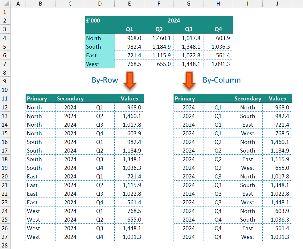
    Description: *//**Unpivot ("flatten") a 2D source array into a vertical data table; each source data point represented as an individual row*//*
                 The main data points are held within a Values column, and the row titles/headers and column headers from the source data table are used to add details as Key and Name columns
    Parameters:
        + data                = (required) An array containing the main data points from the table to unpivot or "flat-file".
        + row_headers         = (required) An array of values which represent the row headers/titles for the main data input array.
                                           The row_headers input array should have the same number of rows as the data input array; there can be one or more columns in the row_headers input array.
        + column_headers      = (required) An array of values which represent the column headers/titles for the main data input array.
                                           The column_headers input array should have the same number of columns as the data input array; there can be one or more rows in the column_headers input array.
        + by_column           = (optional) A True/False input which determines whether the main data input array should be read by column (TRUE), or by row (FALSE).
                                              TRUE = the data array is read by going down each column (top-to-bottom), using the column_headers as the Key column(s) and the row_headers as the Name column(s)
                                             FALSE = the data array is read by going across each row (left-to-right), using the row_headers as the Key column(s) and the column_headers as the Name column(s)
                                           If not supplied, will default to FALSE (therefore reading the data array by row).
        + replace_data_blanks = (optional) A value which can be used to replace any blank data points in the Value column, as per the main data input array.
                                           If the input provided is a number or text string, then this value is used to replace any blank data points.
                                           If the input provided is a logical/Boolean value:
                                              TRUE = blank data points will be replaced with a #N/A error value
                                             FALSE = blank data points will not be replaced
                                           If not supplied, will default to an effective blank string value ( "" ).
        + filter_blanks       = (optional) A True/False input which determines whether to filter out any rows with blank data points within the Values column.
                                           Can be input as TRUE/FALSE (Boolean logical value) or 1/0 (number).
                                           If not supplied, will default to FALSE.
        + filter_errors       = (optional) A True/False input which determines whether to filter out any rows with error values within the data values column.
                                           Can be input as TRUE/FALSE (Boolean logical value) or 1/0 (number).
                                           If not supplied, will default to FALSE.
        + fill_row_blanks     = (optional) Determines whether any blank data points in the row_headers input array should be filled and what value should be used.
                                           The blank cells can be filled with the values from the cells above or below the blank cell, or with a specified value.
                                                +1 = fills the blank data point with the cell value from the row above 
                                                -1 = fills the blank data point with the cell value from the row below
                                                 0 = does not fill the blank values from the input array, instead they are left as an empty string ( "" ) in the output
                                              TRUE = fills the blank data points with the cell value from the row above
                                             FALSE = does not fill the blank values from the input array, instead they are left as an empty string ( "" ) in the output
                                            [text] = any value other than a number or TRUE/FALSE is provided this is used to fill all blank values
                                           If not supplied, will default to FALSE/0
        + fill_column_blanks  = (optional) Determines whether any blank data points in the column_headers input array should be filled and what value should be used.
                                           The blank cells can be filled with the values from the cells to the Left or Right of the blank cell, or with a specified value.
                                                +1 = fills the blank data point with the cell value from the cell to the Left 
                                                -1 = fills the blank data point with the cell value from the cell to the Right
                                                 0 = does not fill the blank values from the input array, instead they are left as an empty string ( "" ) in the output
                                              TRUE = fills the blank data points with the cell value from the cell to the Left
                                             FALSE = does not fill the blank values from the input array, instead they are left as an empty string ( "" ) in the output
                                            [text] = any value other than a number or TRUE/FALSE is provided this is used to fill all blank values
                                           If not supplied, will default to FALSE/0
        + output_vertical     = (optional) A True/False input which determines whether to provide the final output data array in vertical orientation or horizontal orientation.
                                           Can be input as TRUE/FALSE (Boolean logical value) or 1/0 (number).
                                              TRUE = vertical orientation
                                             FALSE = horizontal orientation, running left-to-right across the worksheet
                                           If not supplied, will default to FALSE.
    Error codes:
            #VALUE!     = Occurs when one or more of the inputs provided are invalid.
            #CALC!      = Occurs where the data array dimensions are not the equal to the corresponding dimenesions of the row and column header input arrays.
                          i.e. the row headers array and data array should have the same number of rows 
                               the column headers array and data array should have the same number of columns
    Notes:
        - The replace_data_blanks, filter_blanks, and filter_errors functionality does not consider any blank or error values within the Key column(s) or Name column(s), only the Values column (data array).
        - Additionaly, if the replace_data_blanks option is used, then the filter_blanks option will have no effect on the output as the blank values are replaced before any filtering occurs.
        - If the replace_data_blanks option is used to replace blank data values with #N/A values, then these could then be filtered out by the filter_errors option as the filtering occurs after dealing with blank data points. 
*/
UnPivot = LAMBDA(

    ...

);

The above shows my current preferred format for these Excel Labs AFE modules, making use of multi-line comments to provide the module and function documentation. Using comments in this way for the function documentation allows for more extensive and more verbose information but is only accessible via the Excel Labs add-in. Therefore, I also like to add in the About() function to provide more easily accessible function information on the worksheet.

The initial comment block (lines 1-7) provides the information on the module itself including the suggested module name and version number. I then include the About() function (lines 8-26) followed by the other functions in the order in which I have included them in the About() function information strings.

Each function is declared and defined in the standard Excel Labs AFE way, starting with the function name and ending with a semi-colon:

Function_Name = LAMBDA( ... );

Above each function declaration, I use a multi-line comment block to supply the corresponding function documentation (for example see lines 28-65). This will usually contain:

function name;
function version;
description of the functions action/intended use;
input parameters, including information on:
- whether a parameter is required or optional, and
- the expected input value(s);
potential function output error codes and there meaning; and
any additional notes on how the function is intended to work.

Of note, the description portion of the function documentation is held in its own separate and special comment block. This comment block uses a double asterisk in the format:

/** [Description text] */

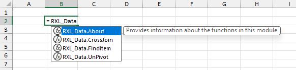
This is important, as the double asterisk comment format indicates to the AFE that this text should be used to populate the Comment property of the defined name that stores the function. As described above the Comment property of the defined function is then displayed to the user when selecting a function to use in their formulae.

Note: The description supplied in the double asterisk comment (“/** … */”) should be a brief description over a single line as there is a 255 character limit for the text stored in the defined name Comment property.

If you wish to use the RXL_Data module (or any other AFE module) in your Excel projects, this can be easily achieved using the below steps:

Ensure that you have the Microsoft Excel Labs add-in installed, and navigate to the Advanced Formula Environment (AFE) tab
In the AFE choose the Modules section from the green ribbon at the top
Click on the “Import from URL” button in the black ribbon (looks like a cloud with a down arrow)

In the dialogue box that pops up enter the GitHub Gist URL for the RXL_Data module (https://gist.github.com/r-silk/e66b3b83363166862c83a5246dc1d3ea)
Before clicking the “Import” button, check the box for “Add formulas to a new module?” and add the suggested module name to the text box that appears.

Once the module has been uploaded, the AFE will save a copy of the full module string complete with code comments in your Excel file, which can then be read via the Excel Labs add-in. The AFE will also save copies of each defined function in the Name Manager as defined names with the specified Comments property, and so you can start using the functions by simply typing =RXL_Data in the formula bar.

27th Apr 2025

Data Analysis Tools (3) – FindItem Function

In February this year I was able to attend the Global Excel Summit 2025 (GES 2025). As was the case at the 2024 Summit, Bob Umlas presented an excellent session show-casing some great Excel tips and tricks. One of things that Bob demonstrated was the idea of finding a value or item within a two-dimensional (2D) array of cells and then returning the relative row and column of that value; in effect the opposite of the INDEX() function or a Lookup function.

e.g. instead of passing a row and column value and returning the value of the cell at that intersection, you can provide the value to find and then return it’s (relative) position.

This seemed like a really fun idea to play around with, so I decided to make my own reverse-INDEX style function: FindItem().

The idea was to build a custom Lambda function where the user could provide a search condition and then return the matching result(s) from an input range. I wanted the search condition to allow for more than just a simple “equals-to” type of match, and I wanted to be able to output either the matching values, the relative position, or the absolute position of the matching cells/values.

As I find is often the case, once I started building my custom function, “feature-creep” came along and I found myself building in all sorts of flexibility and functionality to FindItem(), which I have described below. The full functionality version of the function uses the newer native Excel RegEx functions, but as these may not be available to all users there is also an alternative version of the function which does not use RegEx.

Function Development

The basic principle of the FindItem() function is:

create an output array with the same dimensions as the input range, then;
filter the output array based on the search condition against the original input range; and finally
convert the filtered output array to a single column list of matches.

This approach means that all output conditions can be accommodated at the same point and then filtering can be used to leave only the matching output values.

This does mean there is some loss of efficiency in calculating the output values for all input values, rather than filtering the input values then calculating outputs for only the matching input values. However, the act of filtering the input values based on the search conditions will leave you with only an array of filtered values rather than referenced cells, making calculating the row- and column-type output values more difficult. Instead, these dimensional/positional output values can easily be calculated based on the raw input references at the initial stage of the function calculations.

Having created the array of output values, this is updated to preserve only values where the corresponding input range values match the chosen search condition. Where there is a match the calculated output value is preserved, where there is no match the output array is changed to a #N/A value.

By using this approach of converting non-matching data points in the output array to #N/A values, the filtering and converting to a single column can be achieved with a single TOCOL() function, as the TOCOL() function ignore parameter allows for the exclusion of error values (inc. #N/A) when converting the provided array into a single return column.

Note: This approach means that the FindItem() function can not be used to search/match based on error values as these would be excluded by the TOCOL() function call.

Function Matching Options

I started the FindItem() function development intending to provide simple numeric matching. At its simplest, using the default match_type option, the function will try to match the provided find_item value against each of the values in the input range using “equal-to” logic. I then extended this to also allow “not-equal-to”, “greater-than”, “less -than”, “greater-than-or-equal-to”, and “less-than-or-equal-to” matching logic.

When testing these different matching options, I realised that the default “equal-to” logic could be applied to text/string matching but would only positively return text-based input values which exactly match the whole of the find_item value.

To make the function more useful for text-based searching I added in a new match_type option which could be used for partial text matching, or sub-string searching, on a non-case sensitive basis. I decided to use non-case sensitive matching logic as I felt that this was the more likely option to be useful.

e.g. positively matching the find_item value of “at” in both input values of “battery” and “CATCH“, but not in “car“.

Following the roll-out of the new Excel RegEx functions I decided to also add RegEx searching as a match_type option which would allow for more advanced partial text matching and also give an easy case sensitive search option.

Finally, to make the final function a little more user friendly I made the match_type input parameter capable of accepting either a numeric value or a short string, so that the user can choose the wanted matching logic without having to remember what each input number relates to.

When setting the match_type input parameter you can either use one of the numbers below or enter one of the short string inputs shown below.

Input number	Input text	Match type
`0`	`"="`	(default) equal-to
`1`	`"<>"`	not-equal-to
`2`	`">"`	greater-than
`3`	`"<"`	less-than
`4`	`">="`	greater-than-or-equal-to
`5`	`"<="`	less-than-or-equal-to
`6`	`"find"`	sub-string/partial text match
`7`	`"regex"`	matches the RegEx expression string

Function Output Options

In order to make the function as useful as possible, I wanted to include multiple output options that the user can choose from via the output_type input parameter.

The default output option is to return a list of matching values. This is of most use for text-based matching and for the non-default numeric matching options like “greater-than-or-equal-to” or “not-equal-to”. It can be used for the default “equal-to” matching option but will simply return a list of each matched copy of that value.

As was the main inspiration for the FindItem() function, you can output the position of each match within the input data range. At its simplest the function can output the row-column position of each matching value, either:

relative to the input data range
- e.g. a matching value in the first cell of the input data range would be output as row 1, column 1
relative to the worksheet that the input data range is on
- e.g. a matching value in the first cell of the input data range, where the input range covers cells B2:E5, would be output as row 2, column 2

By default, when using the row-column position output options, the output values are provided in a comma-separated format: [row],[column].

To make the function more useful when using the row-column position output options, the user can set the split_output input parameter to TRUE, and then row-column values for matching values will be output as two separate columns, with the [row] values in the first output column and the [column] values in the second output column. This functionality (splitting the relative positional output) is of most use when matching values within a 2D array of values which have row and column headers, as the FindItem() function outputs can then be used to get the row and column headers for the values which match the search criteria.

As well as providing the row-column position for matching values, the FindItem() function can output the cell address for each matching value within the input data range. This can either be a fully anchored cell address (e.g. $A$1), or unanchored (e.g. A1) but will not include a worksheet name reference. The cell address output option does not allow for R1C1 format cell addresses as these can be constructed from the absolute relative-positional output option if needed, using the row and column position relative to the input data worksheet.

Finally, the FindItem() function can provide a simple count of the number of matches found within the input data range for the provided search criteria.

Input number	Output type
`0`	(default) list of matched values
`1`	relative position [row,col] of each match within the source array
`2`	absolute position [row,col] of each match within the source worksheet
`3`	cell address of each match (A1)
`4`	absolute cell address of each match ($A$1)
`5`	count of matches found

For added presentational option the FindItem() function offers the ability to automatically add header text to the function output via the add_header input parameter. The if_not_found input parameter allows the user to provide a value which is used where the function does not match any of the input range values to the search criteria. By default, if no value is provided for if_not_found then the function will return a #N/A error value, except for when the output_type is set to “count of matches” in which case a value of 0 is returned where there are no matches found in the input range.

Function Code

= LAMBDA(
  // Parameter declarations
  range,
  find_item,
  [match_type],
  [output_type],
  [if_not_found],
  [add_header],
  [split_output],
  // Main procedure
  LET(
    _rng, range,
    _itm, find_item,
    // Deal with the optional input parameters and set default values for any omitted parameters
    _mInp, IF( OR( ISOMITTED(match_type), ISBLANK(match_type)), 0, INT(match_type)),
    _typ, IF( ISNUMBER(_mInp), _mInp + 1, IFNA( MATCH( LOWER(match_type), {"=","<>",">","<",">=","<=","find","regex"}, 0), -1)),
    _optn, IF( OR( ISOMITTED(output_type), ISBLANK(output_type)), 0, INT(output_type)),
    _rep, IF( OR( ISOMITTED(if_not_found), ISBLANK(if_not_found)), NA(), if_not_found),
    _add, IF( OR( ISOMITTED(add_header), ISBLANK(add_header)), FALSE, add_header),
    _splt, IF( OR( ISOMITTED(split_output), ISBLANK(split_output)), FALSE, split_output),
    // Check inputs
    //  --> invalid cell reference in the range parameter will give a #REF! error
    //  --> invalid inputs provided for the match_type or output_type parameters will 
    //      give a #VALUE! Error
    _inpChk, IF(
      NOT(ISREF(range)), 2,
        IF(
          OR(
            _typ < 1, _typ > 8,
            NOT(ISNUMBER(_optn)), _optn < 0, _optn > 5
          ),
        3, 1)
    ),
    // Creates an array of the chosen output type/format to the same dimensions as 
    // the source array
    //  --> the CHOOSE() function determines which output type to use
    _tbl, CHOOSE(_optn + 1,
      _rng,
      (ROW(_rng) - ROW( TAKE(_rng, 1)) + 1) & "," & (COLUMN(_rng) - COLUMN( TAKE(_rng, , 1)) + 1),
      ROW(_rng) & "," & COLUMN(_rng),
      ADDRESS( ROW(_rng), COLUMN(_rng), 4, 1),
      ADDRESS( ROW(_rng), COLUMN(_rng), 1, 1),
      _rng
    ),
    // Calculate the output array
    //  --> the CHOOSE() function determines which match type to use
    //  --> the IF() functions go through the source array and preserves any matches 
    //      (from the created outputs array, _tbl) and sets non-matches to #N/A
    //  --> the TOCOL() function converts the updated array to a single vertical 1D array 
    //      and filters out #N/A values to leave only any matches
    _mtch, TOCOL( 
      CHOOSE(_typ,
        IF(_rng = _itm, _tbl, NA()),
        IF(_rng <> _itm, _tbl, NA()),
        IF(_rng > _itm, _tbl, NA()),
        IF(_rng < _itm, _tbl, NA()),
        IF(_rng >= _itm, _tbl, NA()),
        IF(_rng <= _itm, _tbl, NA()),
        IF( ISNUMBER( FIND( LOWER(_itm), LOWER(_rng))), _tbl, NA()),
        IF( REGEXTEST(_rng, _itm), _tbl, NA())
      ),
    2),
    // Determine whether the return result should be the filtered/matched output array 
    // or the count of the filtered/matched output array
    _calc, IF(_optn <> 5, _mtch, ROWS(_mtch)),
    // Check if the calculated result returns an error suggesting not match 
    // -- if so return the correct "not found" value
    _arr, IF( ISERROR(_calc), IF(_optn = 5, 0, _rep), _calc),
    // Create the required header based on the chosen output type, and stack this on 
    // top of the calculated results array
    _hdr, CHOOSE(_optn + 1,
      "Matches",
      "Row,Column",
      "Row,Column",
      "Cell Address",
      "Cell Address",
      "Count of Matches"
    ),
    _inc, VSTACK(_hdr, _arr),
    // If the relative or absolute cell position output type is chosen and the split_output 
    // parameter is TRUE then the header and results are split into two columns
    _rslt, IF( AND(_splt, _optn > 0, _optn < 3),
      DROP( REDUCE("", _inc, LAMBDA(_acc,_val, VSTACK(_acc, TEXTSPLIT(_val, ",", , TRUE)))), 1),
      _inc
    ),
    // If the add_header parameter is FALSE then remove the header row
    _out, DROP(_rslt, IF(_add, 0, 1)),
    // If there are any #N/A values in the output array these replaced with the 
    // if_not_found value
    _rtn, IF( ISNA(_out), _rep, _out),
    // If the input checks (_inpChk) have flagged then return the required Excel error code, 
    // otherwise return the calculated result (_rtn)
    CHOOSE(_inpChk, _rtn, INDIRECT(""), #VALUE!)
  )
)

The function input parameters are declared in lines 3-9 with the optional parameters defined by the use of square brackets ("[ ]"). This is followed by dealing with the optional parameters setting default values where input values have been omitted (lines 15-22) and then input checks for three of the main input parameters: range, match_type, and output_type (lines 25-33).

As described above, the function first calculates an output array which matches the input data range values in dimensions (lines 37-43), using a CHOOSE() function to determine that chosen output option based on the output_type input parameter.

This is then followed by a combination of a TOCOL() and CHOOSE() functions (lines 51-62):

the CHOOSE() function determines which matching logic to use, with the calculated output values (_tbl) preserved where the corresponding input value matches the search criteria and non-matching values updated to #N/A;
the TOCOL() function then coverts the updated calculated output array to a single column of output values and filters out any non-matching #N/A values.

The next step (line 65) determines whether to output the filtered and converted output array (_mtch) or to provide a count of the number of matches based on the chosen output_type. The filtered and converted output (_calc) is then checked to see if an error is present (suggesting that no matches have been found), in which case either the replacement value (as per if_not_found) is used or a value of 0 is returned if the “count of matches” output option is chosen (line 68).

Appropriate header text is chosen based on the output_type and added to the calculated output (lines 71-79). The header text is added regardless of whether the add_header is True so that it can be correctly split into columns if this option is chosen by the user. If the user has chosen to split the output into two columns, as per the split_output input parameter, then this performed in lines 82-85 but only where a row-column positional output option has been chosen. The TEXTSPLIT() function is used to split the [row],[column] positional output using the "," (comma) character.

If the full output array (_inc) is provided to the TEXTSPLIT() function then only a single column is returned containing the value before the comma (","). By using a REDUCE() function with a VSTACK() to isolate each row of the output array, the TEXTSPLIT() can act on an individual output row, and then stack these split rows back into a single output array with two columns as the output of the REDUCE() function.

After the output array has been split as appropriate, the function considers whether to remove the top header row, based on the add_header input, using a DROP() function (line 87).

Finally, the function checks if any of the input checks have flagged (_inpChk), and if so returns an appropriate error value, otherwise the calculated and updated output array (_rtn) is returned (line 93).

If you want to use the FindItem() function in your own projects, please consider including it via the full RXL_Data module. If you would prefer to include just the single FindItem() function, please use one of the options below:

Using Excel Labs Advanced Formula Environment (AFE) download the RXL_FindItem function using the Gist URL https://gist.github.com/r-silk/ad8fa1536830e6fbfbf91953fa4efc3a
Alternatively, go to the GitHub repository https://github.com/r-silk/RXL_Lambdas and download the file RXL_FindItem.xlsx
- this file contains a copy of the function in the Defined Names which can be copied into your own file
- there is also a “minimised” version of the function which can be copied and pasted directly into the Name Manager when defining a new name of your own — please use the suggested function name of RXL_FindItem
- alternatively, you can use the VBA code and instructions on the “VBA” worksheet to copy the function across to your own project using VBA
- the file contains the documentation for the function as well as some details on development and testing/example usage

20th Apr 2025

Data Analysis Tools (2) – UnPivot Data
Often data within an Excel file will be displayed in a classic (pivot) table format, with a defined two dimensional layout of rows and columns. The rows and columns usually have associated headers/titles and the data within the table may be a summary of some underlying source data using sums or averages.

This data table format is recognised by most users and can make reading and interpretation of the data easier, particularly when looking at values at the intersection of rows and columns. However, working with this type of data, particularly if looking to filter or group the data, can be more difficult.

A common approach within data analysis is to look to un-pivot (or “flatten”) such data tables into a single vertical data table where each row represents a data point and the columns contain the attributes for that data point — data structures such as seen in relational databases or Power Query.

By unpivoting your data into this kind of structure, analysis is easier, especially when applying filtering to the data. The unpivoted data table can also act as a single main data source for any output calculations or charts/visualisations, so that when applying filtering to this one data source it will then be reflected in all outputs that are linked to that data.

For example, with the data shown below, when charting the sales per quarter for a chosen region you could simply use a look-up formula such as XLOOKUP() based on the region required. However, if you wanted to show a detailed comparison by region for a specified quarter then either different look-up formula logic is needed, or a more complex and less efficient formula is requried to allow for both situations dynamically.

If instead, the same data is unpivoted to a flat vertical data table where each row is a single data point and columns are present for region, quarter and year, then simple filtering logic could be used to show either sales across quarters for a specified region or regional performance over a specified quarter, and the change between the two can easily be accomplished.

This data structure also allows for easy interactivity with Slicers and can fairly easily facilitate cross-filtering of an output with multiple Slicers as seen with Power BI style dashboards.

Achieving this kind of unpivoted data table is simple when done manually but can be time consuming and will need updating when the underlying data changes. Alternatively, a more dynamic approach to the unpivoting could be achieved using look-up formulae, but this would likely need manually updating if the structure of the underlying data table is changed, e.g. if rows or columns are added/removed in the underlying data table.

Power Query, once setup, provides a good way to achieve a fully dynamic approach to unpivoting worksheet data whilst allowing for structural and data changes, but requires refreshing of the query for the worksheet output to reflect any source data changes.

This is what inspired me to use a dynamic array-based approach with a custom LAMBDA() function to achieve a fully dynamic and flexible solution to unpivoting my data as standard Excel formulae on the worksheet.

UnPivot() Function

The UnPivot() function takes a two-dimensional (2D) array of data points/values (data input parameter) along with inputs for the associated row headers/labels and columns headers/labels (row_headers & column_headers input parameters). The data points in the main data array are converted to a single column of values and are displayed with the associated row and column headers for each data point. In this way each data point from the source table has its own row and has the useful associated information on the same row in columns next to the data values column.

The row and column header input arrays can be a single row/column or multiple rows/columns allowing for more detailed labelling of each data point and providing more columns on which any filtering or grouping can be applied.

The cells in the data array can be read in a by-row manner (across each row left-to-right) or a by-column manner (down each column top-to-bottom). By default, the data array is read by-row, and the row headers are used as the primary (“Key”) associated label column(s) with the column headers as the secondary (“Name”) label column(s). If the data array is read by-column instead (via the by_column input parameter), then the column headers are used as the primary “Key” column(s) and the row headers as the “Name” column(s).

To make the function more flexible, blank values in the input arrays can be filled or replaced. With the main data array, the replace_data_blanks input parameter can be used to provide a new value, such as a 0 (zero), which is used to replace any blank data points. For the row and column headers, replacing blank values is more complicated. The function allows the user to fill any blank values:
- in the row_headers array with values from the row above or below (via the fill_row_blanks input parameter); and
- in the column_headers array with values from the column to the left or the right (via the fill_column_blanks input parameter).
Filtering can also be applied to the final output to remove any rows where the data values column contains blank cells or Excel error cells, using the filter_blanks and filter_errors input parameters.

Function code
```
= LAMBDA(
  // Parameter definitions
  data,
  row_headers,
  column_headers,
  [by_column],
  [replace_data_blanks],
  [filter_blanks],
  [filter_errors],
  [fill_row_blanks],
  [fill_column_blanks],
  [output_vertical],
  // Main function body/calculations
  LET(
    _dd, data,
    _rh, row_headers,
    _ch, column_headers,
    // Dealing with default values for optional parameters
    _byCol, IF( ISOMITTED(by_column), 0, IF(by_column, 1, 0)),
    _repD, IF( ISOMITTED(replace_data_blanks), "",
      IF( ISLOGICAL(replace_data_blanks),
        IF(replace_data_blanks, NA(), ""),
        replace_data_blanks)
    ),
    _fltrB, IF( ISOMITTED(filter_blanks), 0, IF(filter_blanks, 1, 0)),
    _fltrE, IF( ISOMITTED(filter_errors), 0, IF(filter_errors, 1, 0)),
    _rowB, IF( ISOMITTED(fill_row_blanks), 0, fill_row_blanks),
    _colB, IF( ISOMITTED(fill_column_blanks), 0, fill_column_blanks),
    _vrt, IF( ISOMITTED(output_vertical), 1, IF(output_vertical, 1, 0)),
    // Determine the correct fill direction and if a replacement is string is needed
    // for both the row_headers and column_headers input arrays
    _repR, IF( OR(ISNUMBER(_rowB), ISLOGICAL(_rowB)), "", _rowB),
    _repC, IF( OR(ISNUMBER(_colB), ISLOGICAL(_colB)), "", _colB),
    _dirR, IF( OR(ISNUMBER(_rowB), ISLOGICAL(_rowB)), INT(_rowB), 0),
    _dirC, IF( OR(ISNUMBER(_colB), ISLOGICAL(_colB)), INT(_colB), 0),
    // Input parameter checks
    _inpChk, IFS(
      IFERROR( OR( ROWS(_rh) < 1, COLUMNS(_rh) < 1, ROWS(_ch) < 1, COLUMNS(_ch) < 1, ROWS(_dd) < 1, COLUMNS(_dd) < 1), 3), 3,
      IFERROR( OR( ROWS(_dd) <> ROWS(_rh), COLUMNS(_dd) <> COLUMNS(_ch)), 3), 2,
      TRUE, 1
    ),
    // Assign the row header and column header input arrays to the key columns and name columns arrays depending on the by_column input
    // ensure that assigned key and name column arrays are vertically aligned
    // get the dimensions (rows, columns) of the assigned arrays
    _kCols, IF(_byCol, TRANSPOSE(_ch), _rh),
    _nCols, IF(_byCol, _rh, TRANSPOSE(_ch)),
    _rK, ROWS(_kCols),
    _cK, COLUMNS(_kCols),
    _rN, ROWS(_nCols),
    _cN, COLUMNS(_nCols),
    // Construct the keys (primary) and names (secondary) columns for the output array
    // + The input array is reversed if needed (depending on the direction chosen), and then
    //   a combination of REDUCE(), HSTACK() and SCAN() are used to fill any blanks with an
    //   an appropriate replacement value, one column at a time
    // + The updated input array is returned to it's original direction if needed before being
    //   used in the MAKEARRAY() function to construct the final Keys/Names column.
    _keys, LET(
      _kRep, IF(_byCol, _repC, _repR),
      _kDir, IF(_byCol, _dirC, _dirR),
      _kArr, IF(_kDir = -1, INDEX(_kCols, SEQUENCE(_rK, 1, _rK, -1), SEQUENCE(1, _cK)), _kCols),
      _kFil, DROP( REDUCE(0, SEQUENCE(_cK), LAMBDA(_arr,_col,
        HSTACK(_arr,
          SCAN("", CHOOSECOLS(_kArr, _col),
            LAMBDA(_acc,_val, IF(ISBLANK(_val), IF(_kDir = 0, _kRep, _acc), _val))
          )
        ))),
      , 1),
      _out, IF(_kDir = -1, INDEX(_kFil, SEQUENCE(_rK, 1, _rK, -1), SEQUENCE(1, _cK)), _kFil),
      MAKEARRAY(_rK * _rN, _cK, LAMBDA(_row,_col, INDEX(_out, ROUNDUP(_row / _rN, 0), _col)))
    ),
    _names, LET(
      _nRep, IF(_byCol, _repR, _repC),
      _nDir, IF(_byCol, _dirR, _dirC),
      _nArr, IF(_nDir = -1, INDEX(_nCols, SEQUENCE(_rN, 1, _rN, -1), SEQUENCE(1, _cN)), _nCols),
      _nFil, DROP( REDUCE(0, SEQUENCE(_cN), LAMBDA(_arr,_col,
        HSTACK(_arr,
          SCAN("", CHOOSECOLS(_nArr, _col),
            LAMBDA(_acc,_val, IF(ISBLANK(_val), IF(_nDir = 0, _nRep, _acc), _val))
          )
        ))),
      , 1),
      _out, IF(_nDir = -1, INDEX(_nFil, SEQUENCE(_rN, 1, _rN, -1), SEQUENCE(1, _cN)), _nFil),
      MAKEARRAY(_rK * _rN, _cN, LAMBDA(_row,_col, INDEX(_out, MOD(_row - 1, _rN) + 1, _col)))
    ),
    // Construct the values (data values) column for the output array
    _values, LET(
      _dp, TOCOL(_dd, , _byCol),
      IF( ISBLANK(_dp), _repD, _dp)
    ),
    // Construct the output array
    _rtn, LET(
      _dt, HSTACK(_keys, _names, _values),
      _vl, CHOOSECOLS(_dt, -1),
      // Apply filtering to the constructed output array for blanks and/or errors
      // Note - filtering is only based on the Values (data values) column, 
      //        blanks or error values in the Keys and Names columns will not be filtered
      _dfB, IF(_fltrB, FILTER(_dt, IF( ISERROR(_vl), TRUE, IFNA(_vl, "#") <> "")), _dt),
      _dfE, IF(_fltrE, FILTER(_dfB, NOT(ISERROR( CHOOSECOLS(_dfB, -1)))), _dfB),
      // Transpose the output array if needed
      IF(NOT(_vrt), TRANSPOSE(_dfE), _dfE)
    ),
    // Check if input checks have flagged -- if so return the appropriate error, otherwise return the calculated output array
    CHOOSE(_inpChk, _rtn, LAMBDA(0), #VALUE!)
  )
)
```
The function input parameters are declared in lines 3-12 with the optional parameters defined by the use of square brackets ("[ ]"). This is followed by dealing with the optional parameters setting default values where input values have been omitted (lines 19-29).

Input checks are performed for the three main, and required, input parameters: data, row_headers, and column_headers (lines 37-41).

The main calculated output uses a vertical orientation, i.e. the unpivoted data is converted to a column of data points and output as the “Values” column of the output.

The associated row headers/titles and column headers/titles are assigned to either the primary data column(s) in the output as the “Key” column(s), or the secondary data column(s) in the output as the “Name” column(s). Based on the by_column optional input parameter the user can select whether to unpivot the data by reading down each column of the data array or by default by reading across each row of the data array.

When the by_column option is used, the column headers will make up the primary “Key” columns with the rows as the secondary “Name” columns; otherwise, by default the row headers are used to create the primary “Key” columns and the columns headers used to create the secondary “Name” columns (lines 45-50).

As the unpivoted output array ideally should have no blank values in the “Key” and “Name” columns, the user has the option to fill any blanks via the fill_row_blanks and fill_column_blanks input parameters. The user can choose to:
- provide a new value which is used to fill all blank spaces;
- fill the blank spaces with the value of the cell above (row headers) or to the left (column headers) — input as True/1;
- fill the blank spaces with the value of the cell below (row headers) or to the right (column headers) — input as -1; or
- by default (or an input of False/0), blanks values are not replaced and instead empty strings ("") are used.
Filling in blank header values with the cell value from the row above/column to the left is relatively simple with a SCAN() function. However, it is more challenging when filling with the cell value from the row below/column to the right. To make this process easier, when constructing the “Key” and “Name” columns, if filling from below/right the input array is first reversed (lines 60 & 74), and then the same SCAN() function logic can be used to fill blanks using the previous non-blank value (lines 61-67 & 75-81), before reverting the array back to its original direction as required (lines 68 & 82).

Once the row and column header arrays have been orientated and updated as required, MAKEARRAY() functions are used to construct the “Key” and “Name” columns (lines 69 & 83). This is used to accommodate 2D input arrays (e.g. multiple columns of row headers, or multiple rows of columns headers), and to allow for the production of an effective Cartesian product to label the unpivoted data array, using a similar logic to that used in the CrossJoin() function (see Data Analysis Tools (1) – CrossJoin Lists).

Having created the “Key” and “Name” columns, the data array is converted to a single column using TOCOL(), reading either by column or by row (line 87), and replacing any blank data points as appropriate (line 88).

The main data values column (_values) and the associated data labelling columns (_keys, _names) are stacked together using a HSTACK() function (line 92). The final output is then be filtered to remove any blank data points or Excel error values in the data values column as needed (lines 97-98), and the orientation of the main output can be changed to horizontal (extending across the worksheet) rather than the default of a vertical output if chosen by the user (line 100).

Finally, the function checks if any of the input checks have flagged (_inpChk), and if so, returns an appropriate Excel error value, otherwise the calculated and filtered output array (_rtn) is returned (line 103).

If you want to use the UnPivot() function in your own projects, I encourage you to include it via the full RXL_Data module. If you would prefer to include just the single function, please use one of the options below:
1. Using Excel Labs Advanced Formula Environment (AFE) download the RXL_UnPivot function using the Gist URL https://gist.github.com/r-silk/c31faf1e9de8d01687447bede455f8cc
2. Alternatively, go to the GitHub repository https://github.com/r-silk/RXL_Lambdas and download the file RXL_UnPivot.xlsx
  - this file contains a copy of the function in the Defined Names which can be copied into your own file
  - there is also a “minimised” version of the function, however the minimised function string exceeds the number of characters which can be pasted into the “Refers to” text box of the Name Manager window
  - instead, you can use the VBA code and instructions on the “VBA” worksheet to copy the function across to your own project using VBA
  - the file contains the documentation for the function as well as some details on development and testing/example usage
13th Apr 2025
Data Analysis Tools (1) – CrossJoin Lists
What is a Cross Join?

When working with databases using a language such as SQL, there are times when it is necessary or useful to combine data from different data tables/sources. There are two main ways in which data tables are combined: a JOIN operation, or a UNION operation.
- A UNION will add the rows from one data table to another (concatenation), and where columns are present in both tables these will be combined, otherwise the non-shared columns are included with Null values.
- A JOIN will combine rows from two data tables based on the values in a related column, such as a unique ID column/field. Where a row does not have data present for all columns across both data tables, any missing values are replaced with Null values.
  - INNER JOIN — only returns rows which are present in both data tables based on the related column(s)/field(s)
  - LEFT JOIN — returns all rows from the first (Left) data table and any from the second data table that match to the rows in the first data tale based on the related column(s)/field(s)
  - RIGHT JOIN — returns all rows from the second (Right) data table and any from the first data table that match to the rows in the second data tale based on the related column(s)/field(s)
  - FULL JOIN — returns all rows from both data tables combining those that match based on the related column(s)/field(s) and adding Null values to the unmatched rows
A CROSS JOIN, also referred to as a Cartesian product Join or a Cartesian Join, combines each row from one data table with each row from a second table. This results in a new data table with every possible combination of rows from the input data tables, e.g. if there are five rows in the first input table and 6 rows in the second data table, a CROSS JOIN will produce a new data table with (5 * 6 =) 30 rows.

The CrossJoin() function

I have had a few occasions when it was necessary to be able to model and calculate all combinations of two (or more) input lists within an Excel model.

Creating a single table in Excel containing all combinations of two short lists is a very manual but not too difficult process (see the screenshot of a simple Cartesian Product above). However, for longer lists of inputs or where there are more than two input lists, this can start to become a long and inefficient process. If at any point the user adds extra inputs to any of the lists or makes substantial changes to the input lists, this can lead to a very frustrating and inefficient time updating your calculation table of combinations.

To try to make this process more dynamic and efficient you can use lookup formulae, with or without helper columns, but this can still end up being time consuming if the size of the input lists being combined is changed. Similarly, you could use Power Query to combine the input lists and create the Cartesian product output table and once set up this will be a much more efficient method when any updates are processed to the input lists. However, for a Power Query-based process, updates to the output on the Excel worksheet need to be refreshed and are not triggered simply by the user updating an input cell value.

This inspired me to create a custom LAMBDA() function which would easily allow for the creation of the equivalent of a Cross Join directly on the worksheet which would be entirely dynamic and triggered by a change in an input cell value in the standard manner for a worksheet formula.

Initially the function would deal with a two simple, one-dimensional (1D) vertical lists (i.e. two single columns of variable row length), where each row of the second input array would be added to each row of the first input array. Then enthusiasm lead to the inevitable “feature creep”. As such, the final version of the function allows for:
- input arrays (via the list_one and list_two input parameters) to be of any size and dimensions;
  - The input arrays can a 1D (i.e. a single row or single column) or 2D (multiple rows and columns), and the function will attempt to detect whether the array has a vertical orientation (more rows than columns) or horizontal orientation (more columns than rows).
  - There is additional functionality to allow the user to convert either of the input arrays to a single list / 1D array before the Join, and to do this on a row-first or column-first basis, via the convert_list_one, convert_list_two, list_one_by_column, and list_two_by_column input parameters.
- blank/empty input array cells can be replaced with a given value before the Join, via the replace_blanks input parameter;
- blank/empty rows or rows containing Excel error values in either input lists can be filtered out before the Join, via the filter_blanks and filter_errors input parameters;
- the output array can be filtered to keep only distinct/unique rows, i.e. removing any duplicate combinations of the two input arrays after the Join, via the distinct_rows input parameter; and
- the output array can be forced to either a vertical output (extending down the worksheet) or a horizontal output (extending across the worksheet) via the vertical_output input parameter.
Function code
```
= LAMBDA(
  // Parameter definitions
  list_one,
  list_two,
  [convert_list_one],
  [list_one_by_column],
  [convert_list_two],
  [list_two_by_column],
  [replace_blanks],
  [filter_blanks],
  [filter_errors],
  [distinct_rows],
  [vertical_output],
  // Main function body/calculations
  LET(
    // Dealing with optional parameters
    _cvt1, IF( ISOMITTED(convert_list_one), FALSE, convert_list_one),
    _byCol1, IF( ISOMITTED(list_one_by_column), TRUE, list_one_by_column),
    _cvt2, IF( ISOMITTED(convert_list_two), FALSE, convert_list_two),
    _byCol2, IF( ISOMITTED(list_two_by_column), TRUE, list_two_by_column),
    _rep, IF( ISOMITTED(replace_blanks), "", replace_blanks),
    _blnk, IF( ISOMITTED(filter_blanks), FALSE, filter_blanks),
    _errs, IF( ISOMITTED(filter_errors), FALSE, filter_errors),
    _dst, IF( ISOMITTED(distinct_rows), FALSE, distinct_rows),
    _vrt, IF( ISOMITTED(vertical_output), TRUE, vertical_output),
    // Input checks for the optional parameters and required parameters, returning the _inpChk value as 1-to-3
    _chk, REDUCE(0,
      VSTACK(_cvt1, _byCol1, _cvt2, _byCol2, _blnk, _errs, _dst, _vrt),
      LAMBDA(_acc,_val, _acc + AND( NOT(ISLOGICAL(_val)), NOT(ISNUMBER(_val))))
    ),
    _inpChk, IF(
      OR( NOT(ISREF(list_one)), NOT(ISREF(list_two))), 2,
      IF(_chk > 0, 3,
      1)
    ),
    // Determine if the input array lists are to be considered vertically or horizontally oriented (assumes vertical if square in dimensions)
    //  -- assumes vertical orientation by default, e.g. if there are square dimensions
    _hz1, (COLUMNS(list_one) > ROWS(list_one)),
    _hz2, (COLUMNS(list_two) > ROWS(list_two)),
    // Replace blank values with the replacement string as appropriate
    _list1, IF( ISBLANK(list_one), _rep, list_one),
    _list2, IF( ISBLANK(list_two), _rep, list_two),
    // Re-orientate the input lists if not vertical, and convert to a single vertical 1D array if chosen by the user
    _tbl1, LET(
      _tT, IF(_hz1, TRANSPOSE(_list1), _list1),
      IF(_cvt1,
        TOCOL(_tT, 0, IF(_hz1, NOT(_byCol1), _byCol1)),
        _tT
      )
    ),
    _tbl2, LET(
      _tT, IF(_hz2, TRANSPOSE(_list2), _list2),
      IF(_cvt2,
        TOCOL(_tT, 0, IF(_hz2, NOT(_byCol2), _byCol2)),
        _tT
      )
    ),
    // For the vertical and converted lists, create a filter inclusion list and filter as determined by the user inputs
    _inc1, BYROW(_tbl1, LAMBDA(_row, IF(_blnk, SUM(--(IFNA(_row, "#") <> "")), 1) * IF(_errs, NOT(ISERROR(SUM(_row))), 1))),
    _inc2, BYROW(_tbl2, LAMBDA(_row, IF(_blnk, SUM(--(IFNA(_row, "#") <> "")), 1) * IF(_errs, NOT(ISERROR(SUM(_row))), 1))),
    _fltr1, FILTER(_tbl1, _inc1),
    _fltr2, FILTER(_tbl2, _inc2),
    // Calculate the number of rows and columns for each of the filtered lists
    _rr1, ROWS(_fltr1),
    _rr2, ROWS(_fltr2),
    _cc1, COLUMNS(_fltr1),
    _cc2, COLUMNS(_fltr2),
    // Calculate the output array
    _rtn, LET(
      // Create the repeated lists and stack horizontally
      _cT, HSTACK(
        MAKEARRAY(_rr1 * _rr2, _cc1, LAMBDA(_row,_col, INDEX(_fltr1, ROUNDUP(_row / _rr2, 0), _col))),
        MAKEARRAY(_rr1 * _rr2, _cc2, LAMBDA(_row,_col, INDEX(_fltr2, MOD(_row - 1, _rr2) + 1, _col)))
      ),
      // Limit to unique rows only as required by user inputs
      _dT, IF(_dst,
        UNIQUE(_cT),
        _cT
      ),
      // Transpose the vertical output array to horiztonal (left-to-right) as required by user inputs
      _rT, IF(NOT(_vrt),
        TRANSPOSE(_dT),
        _dT
      ), _rT
    ),
    // Check if an input check has flagged
    //  -- if so, output the appropriate error code
    //  -- if not output the calculated output array
    CHOOSE(_inpChk, _rtn, INDIRECT(""), #VALUE!)
  )
)
```
The function input parameters are declared in lines 3-13 with the optional parameters defined by the use of square brackets ("[ ]"). This is followed by dealing with the optional parameters setting default values where input values have been omitted (lines 17-25).

Input checks are performed for both the two main input parameters (list_one and list_two) and the optional parameters other than the replace_blanks input parameter. As the other optional parameters all have the same required input values (either a logical True/False value, or a single number 0/1), to improve formula efficiency a LAMBDA() function is used to iterate through the optional input parameter values and check their validity via the _chk variable (lines 27-30). This is followed by testing the two required input parameter values via the _inpChk variable (lines 31-35). Preference is given to the required input parameters (list_one, list_two) so that if either has an invalid input value this will be output ahead of any optional input parameter invalid input values.

The main calculations start by determining the orientation of the two input lists (lines 38-39). For each input array:
- if there are more rows than columns the array is considered vertically aligned;
- if there are more columns than rows the array is considered horizontally aligned; and
- where there are an equal number of rows and columns the default is to assume that the array is vertically aligned.
Before the main join calculation is performed, horizontal input arrays are transposed to vertical, and then these vertically aligned input arrays are converted to a single column where this is chosen by the user via the convert_list_one and convert_list_two input parameters (lines 44-57). By default, when converting to a single column array a vertically aligned input array will be read by column and horizontally aligned input arrays will be read by row.

Having converted and aligned the two input arrays (stored in variables _tbl1 and _tbl2), filtering is applied as required as per the filter_blanks and filter_errors input parameters. Initially a filter inclusion array is created using a BYROW() function (lines 59-60), marking rows where all values are blank or where there are any Excel error values present. The filter inclusion list is then used to filter the converted input arrays (lines 61-62).

Note: If the replace_blanks parameter has been used to replace any blank values in the list_one and list_two input arrays (lines 41-42), then the filter_blanks functionality will have not effect as the replacement occurs before the filtering steps.

The Cartesian product of the two aligned, converted, and filtered input arrays is created using MAKEARRAY() functions and combined with a HSTACK() function (lines 71-74). The combined and calculated Cartesian product (_cT), is filtered to distinct combinations only using a UNIQUE() function as required (lines 76-79) and transposed to a horizontal orientation output as required (lines 81-84). By default, a vertical output is preferred, and all calculated output rows are output.

Finally, the function checks if any of the input checks have flagged (_inpChk), and if so, returns an appropriate Excel error value, otherwise the calculated and updated output array (_rtn) is returned (line 89).

If you want to use the CrossJoin() function in your own projects, please consider including it via the full RXL_Data module. If you would prefer to include just the single CrossJoin() function, please use one of the options below:
1. Using Excel Labs Advanced Formula Environment (AFE) download the RXL_CrossJoin function using the Gist URL https://gist.github.com/r-silk/1203fd946f4096f3744083040668dbae
2. Alternatively, go to the GitHub repository https://github.com/r-silk/RXL_Lambdas and download the file RXL_CrossJoin.xlsx
  - this file contains a copy of the function in the Defined Names which can be copied into your own file
  - there is also a “minimised” version of the function which can be copied and pasted directly into the Name Manager when defining a new name of your own — please use the suggested function name of RXL_CrossJoin
  - alternatively, you can use the VBA code and instructions on the “VBA” worksheet to copy the function across to your own project using VBA
  - the file contains the documentation for the function as well as some details on development and testing/example usage
6th Apr 2025
Rolling Calculations for Dynamic Arrays
Sometimes during data analysis, it becomes useful to perform a rolling calculation, also referred to as a running calculation or a moving calculation.

These types of calculations are relatively easy to perform with standard Excel formulas. For example, with a rolling maximum calculation the formula simply compares the current value against the previous maximum value.

As this style of calculation often requires looking back at the previous period output/answer, this can be difficult to implement with dynamic arrays. This is because with Dynamic Arrays, the whole array is calculated in a single step and then output (“spilled”) across the required number of worksheet cells. As such, looking back at a previous output value within the same calculation creates a circular reference.

This circular reference issue can be solved with the use of one of the newer Dynamic Array helper functions, the SCAN() function.

The SCAN() function, takes a starting value and an array, and then traverses that array from left-to-right, top-to-bottom (i.e. by column and then by row / across each row before moving down to the next row). Within the SCAN() function, the actual calculation is performed using a LAMBDA() function which takes two arguments:
- the accumulated output value (_acc in the examples below); and
- the current value from the input array (_val in the examples below)
```
= SCAN([initial_value], [input_array], LAMBDA([_acc],[_val], [calculation))
```
In this way, for a rolling maximum calculation, as the SCAN() function considers each value in the input array it can be compared against the previous calculated result, and the new maximum value is calculated and output.

Rolling Calculations with Dynamic Arrays

One of the advantages of Dynamic Arrays (DA) is their flexibility and their being dynamic(!). As list of input values changes, including increasing/decreasing in number or expanding/contracting in dimensions on the worksheet, by using dynamic arrays as calculation references there is no need to manually update your formulae. Particularly when it comes to staged calculations – where the end-point calculation in your analysis relies on prior calculations rather than directly referencing the inputs – by using a dynamic reference to your inputs and then DA references in all of the calculations, there is no need to update the formulae as the inputs are updated.

As discussed above, the SCAN() function is very helpful here to be able to create such rolling calculations that will work well with arrays, especially DAs. But once any additional functionality is included, such as ignoring blank cells, zero values, non-numeric values, or errors, the calculations can become rather complex and long to write. As such, I wanted to develop dynamic and flexible methods for calculating some common rolling calculations which could then be combined into a single custom LAMBDA() function meaning I wouldn’t need to re-write these formulae each time I wanted to use a rolling calculation.

Rolling SUM()

A rolling SUM() function should be simple to produce as it just requires moving along the input array and adding the current value to the previously calculated total.

With standard (non-DA) Excel formulae this is simple enough to achieve. However, the SUM() function is designed to return a single result making this is more complicated for DAs, as the full array will be input to the SUM() function and then summated together rather than producing the rolling total at each point in the input array.

If instead the addition operator (+) is used between two input arrays (inc. DAs), this will add together the arrays, matching values of the same index in each array, to give a single DA output.

As mentioned above, it is not possible to reference back to the previous calculated result from a DA when calculating that DA output as the full array needs to be calculated before it is output and referenceable, and so this creates a circular reference.

This is where the SCAN() function comes into its own, as it allows for a temporary output variable (the accumulated value variable in the SCAN() function’s LAMBDA()) to be used to store the output result at each stage of the calculation. This temporary variable can be referenced within the main calculation without creating a circular reference as it is effectively separate.

At its simplest, a rolling SUM() function can be created via a simple addition (+ operator) within the LAMBDA() function of the SCAN() to add the accumulated value and the current value. Alternatively, the SUM() function can be used to achieve the same result, and since the introduction of eta-reduced DA helper functions, you can simply replace the LAMBDA() function within the SCAN() function with a direct reference to the function you wish to perform — i.e. just typing SUM as shown below. This means that you don’t need to type out the full LAMBDA() function yourself.

By using the simple + operator and adding some additional logic to the SCAN() function, it is possible to include the intended functionality of being able to ignore non-numeric values, blank cells, and error cells when calculating the rolling total.
```
// Rolling SUM
= SCAN(0, [input array], 
    LAMBDA(_acc,_val, 
        _acc + IF( OR( ISERROR(_val), ISBLANK(_val), NOT(ISNUMBER(_val))), 0, _val)
    )
)
```
Rolling COUNT()

Similar to the SUM() function, the COUNT() function will only return a single output result when provided with an array of input values. Again, the SCAN() function can be used to create a rolling calculation as the input array is traversed. However, when simply using the COUNT() function within the LAMBDA() section of the SCAN() function, especially if using the eta-reduced COUNT keyword, the result is not as might be expected.

This is because, the COUNT() function takes the two LAMBDA() variables (_acc and _val) and counts the number of numeric values between these two variables. The accumulated output value (_acc) is just a single value used as a temporary variable at each stage of the SCAN() main calculation, and the current value accessed by the main SCAN() calculation (_val) is also a single value; in this case the starting value (0) is also a single numeric value. Therefore, at each stage of the main SCAN() calculation, the COUNT() function is only considering two values, meaning that the answer is 2 at each stage.

To change this, you can create your own simple counting logic and then use the SCAN() output to keep a tally of your count.

This also allows for inclusion of the additional logic for the added functionality to exclude zero values, error values, and blank cells from the calculation as wanted as well as only including numeric values like the native COUNT() function.
```
// Rolling COUNT
= SCAN(0, [input array], 
    LAMBDA(_acc,_val, 
        _acc + IF( AND(NOT(ISERROR(_val)), NOT(ISBLANK(_val)), ISNUMBER(_val), IFERROR(_val, 0) <> 0), 1, 0)
    )
)
```
Rolling AVERAGE()

For an accurate rolling/moving average, the average needs to consider all previous values at each stage of the calculation, rather than simply looking back to the previous calculated average and then using that value and the current value to get a new average. With standard Excel formulae this can be achieved easily by using a moving cell reference in the AVERAGE() function with the initial cell reference anchored. However, again the AVERAGE() function returns a single value as the result, and so this approach is not dynamic and will not work for an array, especially a DA, in the manner intended.

Instead, we can use the SCAN() function with one of two potential approaches.
1. Use the SCAN() function to traverse the dimensions of the input array rather than the values of the input array and use this to drive an AVERAGE() function.
- This approach is effective and if used with an AVERAGEIFS() function would allow for the extended functionality (e.g. ignoring zero values, blank cells, etc.). However, it is more complicated to keep fully flexible if allowing for the input array to be either vertically (multiple columns) or horizontally (multiple rows) aligned.
1. Use the SCAN() function with manual average calculation to mimic the result of an anchored, moving range AVERAGE() function.
As I am intending on keeping my custom function as flexible and extendable as possible, and I am already developing methods to calculate the SUM and COUNT of the input array (as described above), I decided to go with the second option.
```
// Rolling AVERAGE -- uses the rolling SUM and COUNT methods from above within a LET() function
= LET(
    _arr, [input array],
    _sum, SCAN(0, _arr, LAMBDA(_acc,_val, _acc + IF(AND(NOT(ISERROR(_val)), NOT(ISBLANK(_val)), IFERROR(_val, 0) <> 0), _val, 0))),
    _cnt, SCAN(0, _arr, LAMBDA(_acc,_val, _acc + IF(AND(NOT(ISERROR(_val)), NOT(ISBLANK(_val)), IFERROR(_val, 0) <> 0), 1, 0))),
    IF(_cnt <> 0, _sum / _cnt, 0)
)
```
Rolling MIN() & Rolling MAX()

For a rolling maximum or minimum value, the calculation required is relatively simple – compare the previous max/min value against the current and output the result. As such, the SCAN() function is ideal as the accumulated/previous output value in the LAMBDA() function can be compared directly against the current input array value using the MAX() or MIN() functions.

When adding the extra functionality of being able to exclude, zero values, blank cells, error cells, and non-numeric values, this is also simple to complete with either some extended logic in the LAMBDA() section of the SCAN() function or by using a MAXIFS() or MINIFS() function in the LAMBDA().

The complication can instead be setting the SCAN() function initial value, as this is a mandatory input parameter for the SCAN() function. For the rolling SUM and rolling COUNT examples above, this input has simply been set to zero (0). However, this could cause incorrect results with the MAX() and MIN() functions:
- If the initial SCAN() function value is 0 and the first input value is 1, then MIN() function comparison of the two would incorrectly give a result of 0 -> the correct result should be 1, as this is the first value in the rolling calculation and so has to be the minimum value in a data set of one value.
- If the initial SCAN() function value is 0 and the first input value is -1, then MAX() function comparison of the two would incorrectly give a result of 0 -> the correct result should be -1, as this is the first value in the rolling calculation and so has to be the maximum value in a data set of one value.
My solution is to find the first appropriate value in the input data set and use this as the SCAN() function initial value, which can be complicated if excluding any non-numeric values, blank cells, error cells, etc.
- e.g. if the first value in the input array is 1, then the SCAN() function initial value is set to 1, meaning that the first MIN()/MAX() comparison of the main calculation would be comparing 1 against 1.
```
// Rolling MIN
= SCAN( INDEX([input array], 1, 1), [input array], 
    LAMBDA(_acc,_val, 
        IF( AND(NOT(ISERROR(_val)), NOT(ISBLANK(_val)), IFERROR(_val, 0) <> 0), MIN(_acc, _val), _acc)
    )
)
// Rolling MAX
= SCAN( INDEX([input array], 1, 1), [input array], 
    LAMBDA(_acc,_val, 
        IF( AND(NOT(ISERROR(_val)), NOT(ISBLANK(_val)), IFERROR(_val, 0) <> 0), MAX(_acc, _val), _acc)
    )
)
```
Custom LAMBDA() function

Having developed ways of dynamically and flexibly calculating my chosen five rolling calculations, the next step is to combine them into a single custom LAMBDA() function, with the user having the ability to choose which output they want. I have also added the ability to exclude blank input cells (using the ignore_blanks input parameter), zero values in the input array (using the ignore_zeros input parameter), and to ignore all error values (using the ignore_errors input parameter).

Note: By default, the function will exclude any #N/A values within the input array from the rolling calculations; any other error values (“# values”) will not be excluded so that potential errors in the input array will follow through to the function output and alert the user. To exclude all errors from the function calculations, use the ignore_errors input parameter.

The custom function is designed to be flexible enough to accept a single dimension (1D) input array (array input parameter) in either vertical or horizontal orientation. By default, the function will return its output array in the same orientation as the input array but can be forced to be output as either a vertical or horizontal array (using the vertical_output input parameter).

To make the custom function more user friendly, the user can enter the calculation input parameter as either a number from 1 to 5 or as short text string (not case sensitive) from an expected list:

number input text input output
1 "sum" rolling SUM calculation
2 "count" rolling COUNT (numeric values) calculation
3 "avg" rolling AVERAGE calculation
4 "min" rolling MIN calculation
5 "max" rolling MAX calculation

RCalc() function

Below is the final combined RCalc() function:
```
= LAMBDA(
  // Parameter declarations
  array,
  calculation,
  [ignore_blanks],
  [ignore_zeros],
  [ignore_errors],
  [vertical_output],
  // Main function body/calculations
  LET(
    // Deal with the calculation parameter input and attempt to match against expected text inputs if the
    // input is not a number
    _num, IF( ISNUMBER(calculation), calculation, IFERROR( MATCH(LOWER(calculation), {"sum","count","avg","min","max"}, 0), 0)),
    // Deal with the optional input parameters and set default values for any omitted parameters
    _igB, IF( ISOMITTED(ignore_blanks), 0, ignore_blanks),
    _igZ, IF( ISOMITTED(ignore_zeros), 0, ignore_zeros),
    _igE, IF( ISOMITTED(ignore_errors), 0, ignore_errors),
    _vOut, IF( ISOMITTED(vertical_output), -1, IF(vertical_output, 1, 0)),
    // Check input validity
    //  --> invalid array input (not a 1D array) will give a #CALC! error
    //  --> invalid calculation, ignore_blanks, or ignore_zeros parameter inputs will give a #VALUE! error
    _inpChk, IF( OR(
      AND( ROWS(array) > 1, COLUMNS(array) > 1),
      ROWS(array) < 1, COLUMNS(array) < 1),
      2,
      IF( OR(
        AND( NOT(ISLOGICAL(_igB)), NOT(ISNUMBER(_igB))),
        AND( NOT(ISLOGICAL(_igZ)), NOT(ISNUMBER(_igZ))),
        AND( NOT(ISLOGICAL(_igE)), NOT(ISNUMBER(_igE))),
        _num < 1, _num > 5),
        3, 1
      )
    ),
    // Determine the orientation of the input data array
    _vrt, ROWS(array) > COLUMNS(array),
    // Filter the input data array for error values, blank cells, and zero (0) values
    _fltE, IF(_igE, IF( ISERROR(array), " ", array), IFNA(array, " ")),
    _fltB, IF(_igB, IF( ISBLANK(array), " ", _fltE), _fltE),
    _fltZ, IF(_igZ, IF((--NOT(ISERROR(array)) * --NOT(ISBLANK(array)) * --(IFERROR(array, " ") = 0)), " ", _fltB), _fltB),
    // Set the initial value for the rolling MIN and MAX calculations
    //  --> uses the value in the array -- if this is not a number then the #N/A is used instead
    //  --> for the SUM, COUNT, and AVERAGE calculations, the starting value is 0 (zero)
    _fst, INDEX(_fltZ, 1, 1),
    _init, IF((--(_fst <> " ") * --NOT(ISBLANK(_fst)) * --(IFERROR(_fst, " ") = 0)), _fst, NA()),
    // Calculate the rolling SUM and COUNT values to be used for the SUM, COUNT, or AVERAGE outputs
    _sum, IF( OR(_num = 1, _num = 3),
      SCAN(0, _fltZ, LAMBDA(_acc,_val, _acc + IF( ISNUMBER(_val), _val, 0))),
      ""
    ),
    _cnt, IF( OR(_num = 2, _num = 3),
      SCAN(0, _fltZ, LAMBDA(_acc,_val, _acc + IF( ISNUMBER(_val), 1, 0))),
      ""
    ),
    // Calculate the chosen output based on the user selected calculation input parameter
    _out, CHOOSE(_num,
      _sum,
      _cnt,
      IF(_cnt <> 0, _sum / _cnt, 0),
      SCAN(_init, _fltZ, LAMBDA(_acc,_val, IFS( AND( ISNA(_acc), ISNUMBER(_val)), _val, ISNUMBER(_val), MIN(_acc, _val), TRUE, _acc))),
      SCAN(_init, _fltZ, LAMBDA(_acc,_val, IFS( AND( ISNA(_acc), ISNUMBER(_val)), _val, ISNUMBER(_val), MAX(_acc, _val), TRUE, _acc)))
    ),
    // Determine whether to force a particular output orientation and transpose the calculated output 
    // as required
    _rtn, IFS(
      _vOut < 0, _out,
      OR(
        AND(_vOut, NOT(_vrt)),
        AND(NOT(_vOut), _vrt)
      ),
      TRANSPOSE(_out),
      TRUE, _out
    ),
    // If the input checks (_inpChk) have flagged then return the required Excel error code, otherwise 
    // return the calculated result (_rtn)
    CHOOSE(_inpChk, _rtn, LAMBDA(0), #VALUE!)
  )
)
```
The function starts by dealing with the calculation input value and determining if a non-number value is passed whether it is one of the expected and allowed text inputs (line 13). This is followed by assessing the optional input parameters and setting default values if any have been omitted by the user (lines 15-18).

Next there is an IF() block which is used to perform input checks. This ensures that the input array passed is valid, the calculation input passed is valid (either a number between 1 and 5 or an allowed string), and that the optional parameter values passed are either a TRUE/FALSE Boolean value or a number (lines 22-33).

The orientation of the initial input array is determined so that the correct orientation can be applied to the output as required (line 35).

To make the combined calculation more efficient, the array of input values (array) is filtered to exclude non-#N/A error values, blank cells, and zero values (_fltZ), as per the optional user inputs (ignore_errors, ignore_blanks, ignore_zeros) rather than including this logic in each of the individual main calculations (lines 37-39). The initial value to be used for the rolling MIN and rolling MAX calculations (_init) is also set (lines 43-44).

The main calculations are performed using broadly the approaches described above and based on the SCAN() function. If the user has selected a rolling SUM or AVERAGE output, then the rolling SUM output is calculated (_sum, lines 46-49). If the user has selected a rolling COUNT or AVERAGE output, then the rolling COUNT output is calculated (_cnt, lines 50-53). The output calculation (_out) is then determined with a CHOOSE() function (lines 55-61)
- if the user has selected a rolling SUM or COUNT output the already calculated output is used (_sum or _cnt);
- if a rolling AVERAGE output is selected then this is calculated using the SUM and COUNT outputs that have already been calculated (_sum/_cnt);
- if a rolling MIN or MAX output is selected then this is calculated using the SCAN() function approach as above.
Having chosen and calculated the required output array, the function determines whether the output array orientation needs to be changed to fit with the user input (lines 64-72).

Finally, the function checks whether an input check was flagged (line 75), in which case the appropriate Excel error code is returned as the final function output, otherwise the updated calculated output array (_rtn) is returned.

If you want to use the RCalc() function in your own projects or custom functions, please use one of the options below:
1. Using Excel Labs Advanced Formula Environment (AFE) download the RXL_RCalc function using the Gist URL https://gist.github.com/r-silk/b124f8468b1615a40b42feda7545bc0a
2. Alternatively, go to the GitHub repository https://github.com/r-silk/RXL_Lambdas and download the file RXL_RCalc.xlsx
  - this file contains a copy of the function in the Defined Names which can be copied into your own file
  - there is also a “minimised” version of the function which can be copied and pasted directly into the Name Manager when defining a new name of your own — please use the suggested function name of RXL_RCalc
  - the available file contains the documentation for the function as well as some details on development and testing/example usage
30th Mar 2025

Excel Bits & Pieces

Category: Lambdas

Data Analysis Tools (4) – Function Module

Data Analysis Tools Module (RXL_Data)

Data Analysis Tools (3) – FindItem Function

Function Development

Function Matching Options

Function Output Options

Function Code

Data Analysis Tools (2) – UnPivot Data

UnPivot() Function

Function code

Data Analysis Tools (1) – CrossJoin Lists

What is a Cross Join?

The CrossJoin() function

Function code

Rolling Calculations for Dynamic Arrays

Rolling Calculations with Dynamic Arrays

Rolling SUM()

Rolling COUNT()

Rolling AVERAGE()

Rolling MIN() & Rolling MAX()

Custom LAMBDA() function

`RCalc()` function

number input	text input	output
`1`	`"sum"`	rolling `SUM` calculation
`2`	`"count"`	rolling `COUNT` (numeric values) calculation
`3`	`"avg"`	rolling `AVERAGE` calculation
`4`	`"min"`	rolling `MIN` calculation
`5`	`"max"`	rolling `MAX` calculation

Category: Lambdas

Data Analysis Tools (4) – Function Module

Data Analysis Tools Module (RXL_Data)

Data Analysis Tools (3) – FindItem Function

Function Development

Function Matching Options

Function Output Options

Function Code

Data Analysis Tools (2) – UnPivot Data

UnPivot() Function

Function code

Data Analysis Tools (1) – CrossJoin Lists

What is a Cross Join?

The CrossJoin() function

Function code

Rolling Calculations for Dynamic Arrays

Rolling Calculations with Dynamic Arrays

Rolling SUM()

Rolling COUNT()

Rolling AVERAGE()

Rolling MIN() & Rolling MAX()

Custom LAMBDA() function

RCalc() function

`RCalc()` function